Compare IW wavelets with classical wavelets: linear approximation of signals¶

The Python File User_Example2.py can be downloaded. It runs the code of this tutorial.

We now compare classical wavelet decomposition with intertwining wavelets (IW wavelets) studying linear approximation of signals. The goal is to understand intertwining wavelets properties with respect to classical wavelets ones. In particular we want to check if intertwining wavelets have the classical properties we expect from a wavelet basis, especially the fact that the detail part is “small” whenever the signal has some regularity.

To avoid confusion we have to say that there is no fast algorithm to compute intertwining wavelet coefficients (even if the toolbox iw was optimized as much as we could) and their computation is based on basic linear algebra.

We work with the file Torus_1024

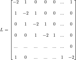
This graph connects each of its 1024 vertices with two neighbours. Its laplacian matrix is

$L = \begin{bmatrix} -2 & 1 & 0 & 0 & 0 & ... & 1\\\\ 1 & -2 &1 & 0 & 0 &... & 0\\\\ 0 & 1 &-2 & 1 & 0 &... & 0\\\\ 0 &0 &1 &-2& 1& ...& 0\\\\ ... &... &... &...& ...& ...& 0\\\\ 1& 0 &... &...& ...& 1& -2 \end{bmatrix}$

We start with a quick description of the outputs of the main class IntertwiningWavelet and show how to process a signal.

Getting started¶

Load Python modules

The following Python modules should be useful.

scipy.sparse since we will use sparse matrices,
NumPy since we will process matrices and arrays,
matplotlib.pyplot for vizualisation

>>> import numpy as np
>>> import scipy.sparse as sp
>>> import matplotlib.pyplot as plt

Load the graph file

>>> from iw.data.get_dataset_path import get_dataset_path
>>> graph_file = get_dataset_path("tore_1024.g")

Start the instances of IntertwiningWavelet

>>> from iw.intertwining_wavelet import IntertwiningWavelet
>>> iw = IntertwiningWavelet(graph_file)
"The graph is reversible the pyramide algorithm....
                can proceed"
>>> iw.pretreatment # To check if the graph has the required reversibility (symmetry)
True

Process the method

Here we choose to set the approximate cardinal of the set of approximation coefficients.

>>> iw.process_analysis(mod='card', m=512) # To have at most 512 approximation coefficients.
>>> print(iw.process_analysis_flag) # True if the decomposition process has been done.
True

Graphs and subgraphs¶

We start with the main attribute tab_Multires of iw which contains the sequence of subgraphs and which also contains the basis.

>>> tab = iw.tab_Multires # Attribute with all the analysis structure

The variable tab is a MemoryView which has three attributes

>>> print(tab)
<iw.multiresolution.struct_multires_Lbarre.Tab_Struct_multires_Lbarre object at 0x7f3186287e30>

The attribute steps: it is the number of decomposition levels.

>>> print(tab.steps) # To get the number of decomposition levels
2

The attribute Struct_Mres_gr: it is the sequence of subgraphs which is as well a MemoryView. You can access to the different levels as follows

>>> subgraphs = tab.Struct_Mres_gr # To get the sequence of subgraphs
>>> j0 = 0
>>> Sg = subgraphs[j0] # To get access to the subgraph at level j0+1

At each level j0 it is possible to get

the list of vertices of the next subgraph. It is again a MemoryView to save memory. You can access the information using NumPy

>>> >>> # Indices of the vertices of the subgraph: drawn from the vertices of the seminal graph
>>> ind_detailj0=np.asarray(Sg.Xbarre)

Watch out that if the level is not j0 = 0 but j0>0 the indices in Sg.Xbarre are taken among the set {0,.. nbarre-1} with nbarre the cardinal of the number of vertices of the graph at level j0-1. In other words the set Sg.Xbarre is not given as a subset of the vertices of the original graph, but of the graph it was drawn from. The following code can be used.

>>> if j0>0: # To recover the indices in the original graph if j0>0
        for i in range(j0-1,-1,-1):
            Xbarrei=np.asarray(subgraphs[i].Xbarre)
            ind_detailj0=Xbarrei[ind_detailj0].copy()

the Laplacian matrix encoding the weights of the subgraph. It is the laplacian of a continuous Markov chain, so this is a matrix based on the vertices of the subgraph and whose non diagonal entries are $w(x,y)\geq 0$ and diagonal entries are $w(x) = -\sum\limits_{x\neq y}w(x,y)$

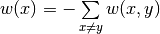
You can access to it as a sparse matrix. The fields Sg.rowLbarres, Sg.colLbarres, Sg.shapeLbarres allow it.

>>> Lbarre0s = Sg.Lbarres
>>> print(Lbarre0s) # It is again a MemoryView
<MemoryView of 'ndarray' object>
>>> # Let us get the sparse matrix
>>> Lbarre0ms =  sp.coo_matrix((Lbarre0s,( Sg.rowLbarres, Sg.colLbarres)),
    shape=(Sg.shapeLbarres, Sg.shapeLbarres))

>>> plt.figure() # Let us visualize the non vanishing coefficients
>>> plt.spy(Lbarre0ms, markersize=2)
>>> plt.title('Localization of non vanishing entries at level '+str(j0+1))
>>> plt.xlabel('Indices')
>>> plt.show()

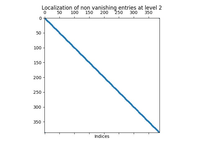
Localization of the non vanishing coefficients of the Laplacian of the subgraph at level j0+1.¶

Watch out that the laplacian matrix of the graph is computed through a sparsification step from another Laplacian matrix, the Schur complement of the original laplacian, which is also stored in Sg under the field Sg.Lbarre

>>> Lbarre0 = Sg.Lbarre
>>> print(Lbarre0) # It is again a Memory view
<MemoryView of 'ndarray' object>
>>> # Let us get the sparse matrix
>>> Lbarre0m = sp.coo_matrix((Lbarre0,( Sg.rowLbarre, Sg.colLbarre)),
    shape=(Sg.shapeLbarre, Sg.shapeLbarre))
>>> sp.linalg.norm(Lbarre0m-Lbarre0ms) # check the difference between the Schur complement and its sparsified version
0
>>> # Here the Schur complement and its sparsified version are the same

Analysis and reconstruction operators¶

We come back to the attributes of tab.

The third attribute of tab is Struct_Mana_re. It stores the analysis operator to compute the wavelet coefficients and the reconstruction operators to compute a signal given its coefficients. It is again a MemoryView object

>>> basis = tab.Struct_Mana_re
>>> print(basis)
<MemoryView of 'ndarray' object>
>>> l0 = 0 # To access to the functions of the first level (finest scale)
>>> a0 = basis[l0]

The attributes of basis store all the operators needed to analyse signals, ie. to compute wavelets coefficients, and the operators to reconstruct the signals given coefficients.

These objects beeing slightly more complicated to handle and not really useful in this experiment we do not explore them now more in details. If you want to know more there is a dedicated tutorial Analysis and reconstruction.

Linear approximation of signals¶

Process a signal¶

We will now compute the intertwining wavelet (IW) coefficients of a signal and its decomposition in a classical wavelet basis (CW).

Signal input¶

This is the classical model commonly used in the reference book by S. Mallat “A wavelet tour of signal processing”, Academic press.

>>> adr_signal = get_dataset_path("signal1D.mat")
>>> Sig = np.loadtxt(adr_signal)  # download the signal
>>> Sig_iw = np.reshape(Sig,(1,n)) # reshape Sig in a 2d array to be able to run iw

Let us have a look on it

>>> plt.figure()
>>> plt.plot(Sig_iw[0,:]) # Watch out that Sig_iw is a 2d NumPy array
>>> plt.title('Original signal')
>>> plt.show()

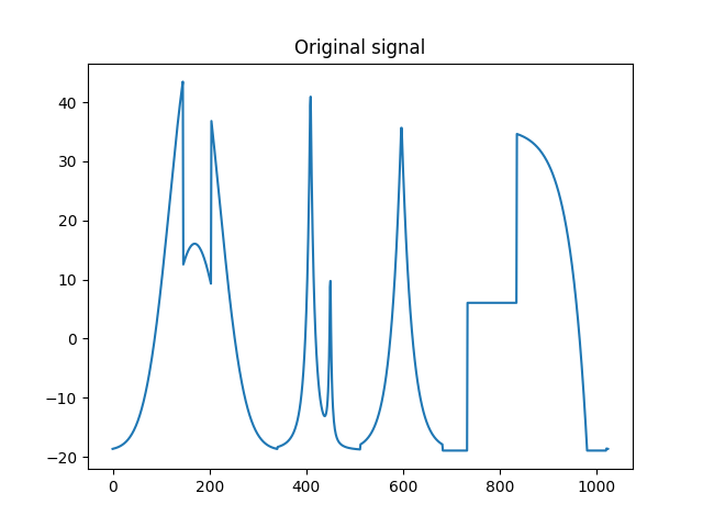
Original signal.¶

IW coefficients¶

Computation of the intertwining wavelet coefficients

We compute the intertwining wavelet coefficients using the attribute of iw which is process_coefficients. The output is a 2d NumPy array, with possibly one line.

>>> coeffs_iw = iw.process_coefficients(Sig_iw)
>>> print(coeffs_iw.shape)
(1, 1024)
>>> plt.figure()
>>> plt.plot(coeffs_iw[0,:],'*') # Watch out that coeffs is a 2d NumPy array
>>> plt.title('Intertwining wavelet coefficients')
>>> plt.show()

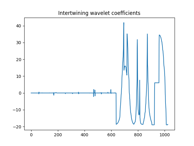
Intertwining wavelet coefficients.¶

Watch out that the Intertwining basis is not orthonormal, and especially the basis vectors are not normalised.

Organization of the coefficients:

The organization of the coefficients in the NumPy array coeffs_iw is as follows

coeffs_iw $=[[g_1,g_2,\dots,g_K,f_K]]$

with

$g_1$ : the sequence of coefficients of the finest details level,
$g_K$ : the sequence of coefficients of the coarsest details level,
$f_K$ the sequence of scaling coefficients, or so called approximation coefficients.

The attribute following_size of iw gives the number of coefficients in each layer

>>> levels_coeffs = np.asarray(iw.following_size)
>>> print(levels_coeffs)
[440 197 387]

In our example

the finest details level $g_1$ has 440 coefficients,
the coarsest details level $g_2$ has 197 coefficients
we have 387 approximation coefficients in $f_2$ .

Remember our method is based on a random subsampling and thus the number of coefficients in each layer generally changes at each new run of iw. But we compute a basis and thus the total number of coefficients is always the total number of vertices in the graph.

CW coefficients¶

Computation of classical wavelet coefficients

Use your favorite codes and your favorite wavelet basis to compute classical wavelet coefficients. Here we work with PyWavelets

>>> # import the PyWavelet toolbox
>>> import pywt

Choose your scaling function

>>> ond='db4'

Compute the wavelet coefficients

>>> # Reshape the signal to have a simple array
>>> Sig_o=Sig.copy()
>>> Sig_o=np.reshape(Sig_o,(n,))
>>> # Compute the wavelet coefficients
>>> Ca,Cd = pywt.wavedec(Sig_o, ond, level=1,mode = "periodization")

Let us look at the coefficients

>>> coeffs_cw=np.concatenate((Cd,Ca))
>>> plt.figure()
>>> plt.plot(coeffs_cw)
>>> plt.title('Classical wavelet coefficients')
>>> plt.show()

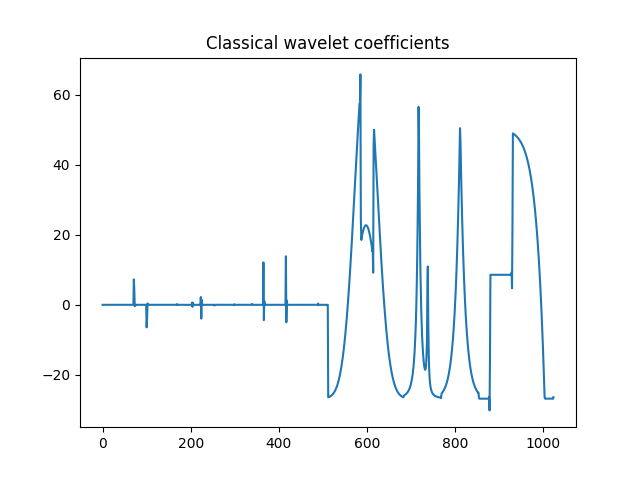
Classical wavelet coefficients.¶

Linear approximation¶

By linear approximation of a signal, we mean here the approximation of a signal obtained by putting all the detail coefficients to 0. This amounts to project the signal on a vector space which does not depend on the chosen signal.

Let us emphasize that projections through IW are not orthogonal in general.

We compare the linear approximations computed using the classical wavelet decomposition and using intertwining wavelet decomposition. Recall that we have 512 classical wavelet scaling coefficients and 387 intertwining wavelet scaling coefficients (in this experiment).

Linear approximation computed with scaling coefficients

Let compute it with intertwining wavelets (or so called IW).

>>> coeffs_approx_iw = np.zeros((1,n))
>>> napprox = levels_coeffs[tab.steps]
>>> coeffs_approx_iw[0,n-napprox:n] = coeffs_iw[0,n-napprox:n].copy() # all the detail coefficients are set to 0
>>> plt.figure()
>>> plt.plot(coeffs_approx_iw[0,:],'*')
>>> plt.title('coefficients of the iw approximation part')
>>> plt.show()

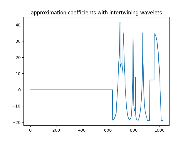
Approximation part coefficients computed with iw: only the 387 scaling coefficients are kept.¶

Let us compute the approximation part from its IW coefficients

>>> approx_iw = iw.process_signal(coeffs_approx_iw)
>>> plt.figure()
>>> plt.plot(approx_iw[0,:])
>>> plt.title('Approximation part with iw')
>>> plt.show()

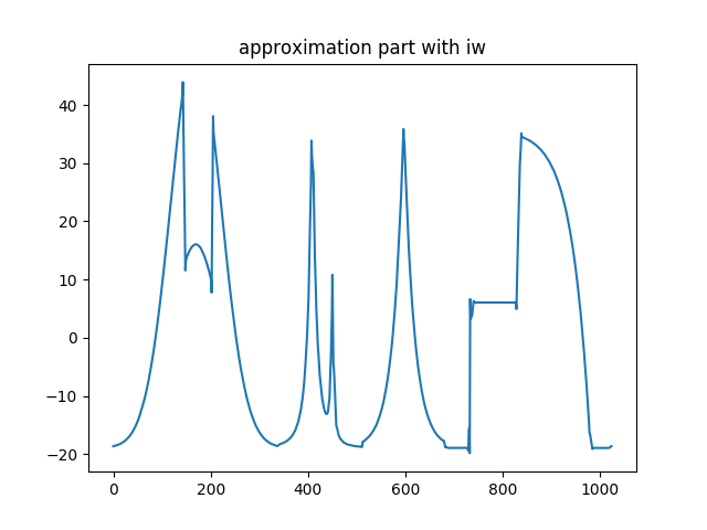
Approximation part with intertwining wavelets.¶

Let compute a linear approximation with classical wavelets (or so called CW).

>>> Ca_approx=Ca.copy()
>>> Cd_approx=np.zeros(Cd.shape)
>>> coeffs_cw=[Ca_approx,Cd_approx]
>>> approx_cw=pywt.waverec(coeffs_cw, 'db4',mode =  "periodization")
>>> plt.figure()
>>> plt.plot(approx_cw)
>>> plt.title('Approximation with classical wavelets')
>>> plt.show()

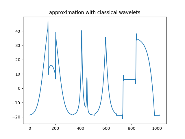
Approximation part with classical wavelets.¶

Compare the two approximations

>>> approx_iw=np.reshape(approx_iw,(n,))
>>> plt.figure()
>>> plt.subplot(2,1,1)
>>> plt.plot(approx_cw) # on top approximation with the classical wavelets
>>> plt.subplot(2,1,2)
>>> plt.plot(approx_iw) # below approximation with iw
>>> plt.show()

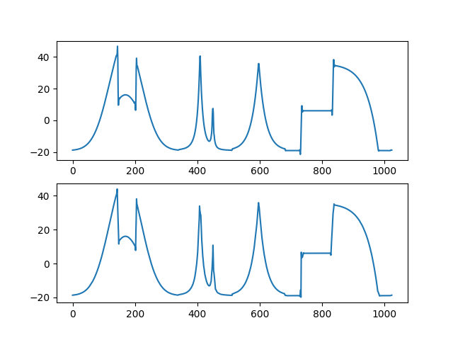
Comparison of the approximation part computed with classical wavelets (on top) and with intertwining wavelets (bottom).¶

Watch out that intertwining wavelets have only one vanishing moment and we can not guarantee the regularity of the reconstruction functions. What we can prove is that a Jackson type inequality is satisfied: whenever the signal is regular we expect the detail contribution to be small.

>>> plt.figure()
>>> plt.subplot(2,1,1)
>>> plt.plot(Sig_o) # # on top the original signal
>>> plt.subplot(2,1,2)
>>> plt.plot(Sig_o-approx_iw) # below the difference between the original signal and the IW approximation part
>>> plt.show()

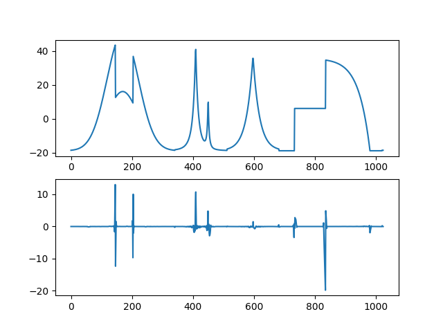
../_images/ex2_compare_approx_detail_iw_1024.png

On top the original signal, bottom the detail part computed by iw.¶

Let us compute the relative error we have when we replace the signal by its approximation (IW approximation or CW approximation)

>>> print(np.linalg.norm(Sig_o-approx_iw)/np.linalg.norm(Sig_o))
0.07732780634701093
>>> print(np.linalg.norm(Sig_o-approx_cw)/np.linalg.norm(Sig_o))
0.040548434074767645

As you can see the relative errors are of the same order although the IW approximation is computed with 387 approximation coefficients whereas the classical wavelet approximation is computed with 512 approximation coefficients !