Run IntertwiningWavelet on other standard graphs: the Minnesota¶

We now use iw and run it on a standard graph: the Minnesota road network. Our goal will be to study a step function on this graph and compute a non linear approximation of it.

We will use the Toolbox PyGSP since it uses the weight matrix as a starting point to encode the graph, just as we do. We will use as well the visualization tools of PyGSP.

Feel free to use instead any of your favorite tool !

The Python File User_Example5.py can be downloaded to run the code of this tutorial. A function is required to write .g files and you find it in the file write_dot_g_sparse.py.

We start with a quick description of the outputs of the main class IntertwiningWavelet and show how to process a signal.

Getting started¶

Download modules¶

Load Python modules

The following Python modules should be useful.

scipy.sparse since we will use sparse matrices,
NumPy since we will process matrices and arrays,
matplotlib.pyplot for visualization

>>> import numpy as np
>>> import scipy.sparse as sp
>>> import matplotlib.pyplot as plt

Load PyGSP modules

>>> from pygsp import graphs, filters, plotting

Load a module to write a .g file

We need a function to write from a matrix the .g file used by iw.

You can download an example of such a function here write_dot_g_sparse.py (courtesy B. Stordeur).

This works with a sparse adjacency matrix as it is the case with PyGSP.

>>> from write_dot_g_sparse import write_gsp_to_g

Load a graph¶

Graph input

Here we choose the Minnesota road map as a graph computed by PyGSP

>>> G = graphs.Minnesota()
>>> n = G.N # to have the number of vertices
>>> print(n)
2642

Graph visualization

We can have a look at it

>>> G.plot(vertex_size=30)

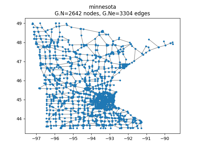
Minnesota road map as a graph.¶

Write the .g file

Remember iw runs with .g type files.

>>> W=G.W # Extract the weight matrix of the graph

>>> # write the .g file to run iw
>>> graph_g = 'Minnesota.g'
>>> write_gsp_to_g(W,graph_g)

Start the instances of IntertwiningWavelet

>>> from iw.intertwining_wavelet import IntertwiningWavelet
>>> iw = IntertwiningWavelet(graph_g)
"The graph is reversible the pyramide algorithm....
                can proceed"
>>> iw.pretreatment # To check if the graph has the required reversibility (symetry)
True

Run the method¶

Here we choose to keep at most 5% of IW coefficients to be approximation coefficients (about 132 approximation coefficients), which means that we have about 95 % of IW coefficients which are detail coefficients.

>>> # To have at most 132 approximation coefficients.
>>> iw.process_analysis(mod='card', m=132)
>>> print(iw.process_analysis_flag) # True if the decomposition process has been done.
True
>>> tab = iw.tab_Multires # Attribute with all the analysis structure

Process a step signal¶

We will now compute the intertwining wavelet (IW) coefficients of a step signal defined and studied in [cit4] as well as in our article [cit2].

Step signal¶

Signal input

>>> G.compute_fourier_basis()
>>> vectfouriers = G.U;
>>> Sig = np.sign(vectfouriers[:,1])

Let us have a look on it

>>> plt.set_cmap('jet')
>>> si = 10
>>> G.plot_signal(Sig,vertex_size=si)

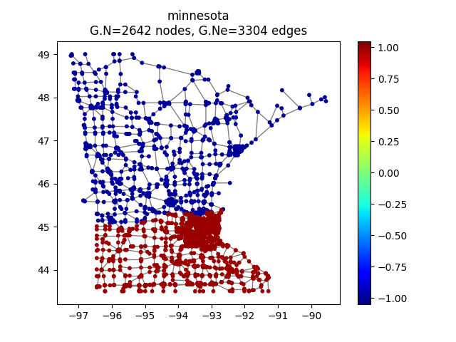
Original signal.¶

IW coefficients¶

Computation of the intertwining wavelet coefficients

We compute the intertwining wavelet coefficients using the attribute of iw which is process_coefficients. The output is a 2d NumPy array, with possibly one line.

>>> # Reshape the signal to have it as a row matrix
>>> Sig_iw=np.reshape(Sig,(1,n))
>>> coeffs_iw = iw.process_coefficients(Sig_iw)

Organization of the coefficients:

The organization of the coefficients in the NumPy array coeffs_iw is as follows

coeffs_iw $=[[g_1,g_2,\dots,g_K,f_K]]$

with

$g_1$ : the sequence of coefficients at the finest details level,
$g_K$ : the sequence of coefficients at the coarsest details level,
$f_K$ the sequence of scaling coefficients, or so called approximation coefficients.

The attribute following_size of iw gives the number of coefficients in each layer

>>> levels_coeffs = np.asarray(iw.following_size)
>>> print(levels_coeffs)
[762 540 372 242 168 137  88  66  87  58 122]

Remember our method is based on a random subsampling and thus the number of coefficients in each layer generally changes at each new run of iw. But we compute a basis and thus the total number of coefficients is always the total number of vertices in the graph.

In our example

the finest details level $g_1$ has 762 coefficients,
the coarsest details level $g_K$ has 58 coefficients
we have 122 approximation coefficients in $f_K$ .

Approximation component¶

Our signal is the sum of two main components: the approximation part and the detail part. Let us have a look at the approximation component.

We reconstruct the signal whose wavelet coefficients are $[0...0,f_K]$ . This means that all the detail coefficients vanish.

>>> coeffs_approx_iw = np.zeros((1,n))
>>> napprox = levels_coeffs[tab.steps]

>>> # we keep only the f_K coefficients.
>>> coeffs_approx_iw[0,n-napprox:n] = coeffs_iw[0,n-napprox:n].copy()

Let us compute the approximation part from its IW coefficients

>>> approx_iw = iw.process_signal(coeffs_approx_iw)

Let have a look at it

>>> G.plot_signal(approx_iw,vertex_size=si)

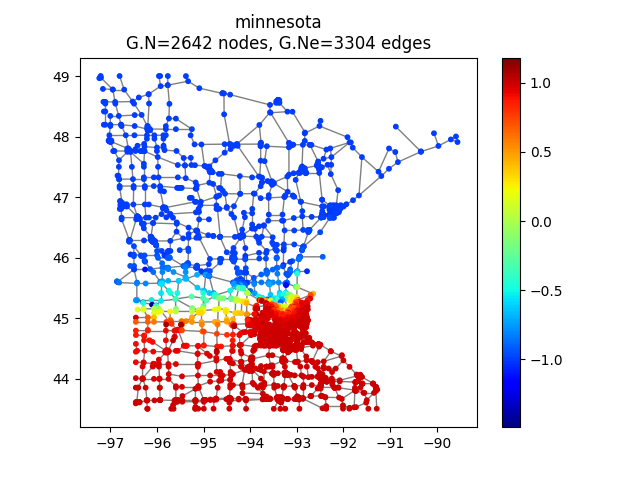
Approximation part with intertwining wavelets.¶

The approximation component is smoother than the original signal, as was expected.

Non linear approximation¶

We threshold the coefficients by keeping the n_T largest detail coefficients and reconstruct the thresholded signal. We will keep the approximation coefficients and will not threshold it.

Thresholding IW coefficients¶

Normalization of intertwining wavelet coefficients

Our basis functions are not orthogonal and even not normalized. To threshold the coefficients an option is to normalize them in order to fix a way of comparing the size of the coefficients. There are several strategies one can choose.

We propose here the following scheme and we want to emphasize that one could choose another option.

Let us call $\psi_k$ our basis functions. In other words the coefficients of a signal $f$ are computed through the formula $d_k=\langle f,\psi_k\rangle_\mu$ .

Recall that our setting allows to have a non uniform reversibility measure $\mu$ and we need to use the appropriate scalar product

$\langle .,.\rangle_\mu:(f,g)\mapsto \sum\limits_{x=0}^{n-1}f(x)g(x)\mu(x)$ .

But if the Laplacian matrix $L$ is as it is often the case symetric then the scalar product $\langle .,.\rangle_\mu$ is the canonical one.

Since the functions of our basis $\{\psi_k,k\in [0,n-1]\}$ are non orthogonal but a linear independent system we can compute a family of functions $\widetilde{\psi_k}$ such that for each $k$ , $\langle \widetilde{\psi_k},\psi_k\rangle_\mu=1$ and for each $k\neq k'$ , $\langle \widetilde{\psi_k},\psi_{k'}\rangle_\mu=0$ . This is called in general the dual system of the $\{\psi_k,k\in [0,n-1]\}$ . The signal $f$ is given by

$f =\sum\limits_k \langle f,\psi_k\rangle_\mu \widetilde{\psi_k}$

Our strategy is to compute 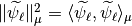$\|\widetilde{\psi_\ell}\|^2_\mu=\langle \widetilde{\psi_\ell},\widetilde{\psi_\ell}\rangle_\mu$ .

Then in a second step for each detail coefficient $d_\ell$ we will store $d_\ell\|\widetilde{\psi_\ell}\|_\mu$ and sort it. Since we will not threshold the approximation coefficients we do not normalize the approximation coefficients.

This is processed through the following function.

# to compute the mu-norm of the m first reconstruction functions
def norm_psi_tilde(m,mu):

    # this matrix is the matrix of the iw-coefficients of the psi_tilde system
    coeffs_dir = np.eye(m,n)

    # (without the functions related to the approximation)

    # compute the psi_tilde family
    #(without the approximation reconstruction functions)
    psi_tilde = iw.process_signal(coeffs_dir)

    # compute the collection of norms of the psi_tilde vectors
    norm_psi_tilde = np.linalg.norm(psi_tilde*np.sqrt(mu),axis=1)

    return norm_psi_tilde

We apply this function and compute $\|\widetilde{\psi_\ell}\|_\mu$ for all detail functions ( $\ell=0,\dots,n-$ napprox).

>>> n = np.size(coeffs_iw) # This yields the total number of coefficients

>>> # to get the sequence of coefficient's number by level
>>> levels_coeffs = np.asarray(iw.following_size)

>>> # to get the number of approximation coefficients
>>> napprox = levels_coeffs[tab.steps]

>>> # We want to compute all the norms of the detail functions
>>> m = n-napprox

>>> # iw gives the reversibility measure which is the uniform measure if L is symetric

>>> mu = np.asarray(iw.mu_initial)

>>> mu_r = np.reshape(mu,(1,n))/np.sum(mu) # we work with a row vector.
>>> n_psi_tilde = norm_psi_tilde(m,mu_r)

Let us visualize it. We can see clearly that our functions are not normalized.

../_images/norms_detail_psitilde_Minnesota.png

Norms $\|\widetilde{\psi_\ell}\|_\mu$ for all detail reconstruction functions.¶

Thresholded signal¶

Compute the thresholded signal

We have now to compute $d_\ell\|\widetilde{\psi_\ell}\|_\mu$ and sort them before computing the thresholded signal. All of this is done using the following function.

def non_linear_iw(sig,nT,coeffs_iw,n_psi_tilde):
    n = np.size(coeffs_iw) # This yields the total number of coefficients

    # to get the sequence of coefficient's number
    levels_coeffs = np.asarray(iw.following_size)

    # to get the number of approximation coefficients
    napprox = levels_coeffs[tab.steps]

    # compute the number of the approximation coefficients
    m=n-napprox

    coeffs_iwT = coeffs_iw.copy()
    coeffs_iwn = coeffs_iwT[0,0:m].copy()*n_psi_tilde

    # we sort the detail coefficients
    arg_iwT = np.argsort(np.abs(coeffs_iwn))

    # we keep only the nT largest detail coefficients
    coeffs_iwT[0,arg_iwT[0:m-nT]] = np.zeros((1,m-nT))

    # Reconstruct the signal
    sig_nT=iw.process_signal(coeffs_iwT)

    return sig_nT

We now compute the signal with $n_T$ non vanishing detail coefficients and vizualize it. Here we compute this non linear approximation with about 15 % of the coefficients of the original signal. The non vanishing coefficients are for about 5% approximation coefficients and 10 % are detail coefficients.

>>> nT = 260
>>> Sig_iw_nT = non_linear_iw(Sig_iw,nT,coeffs_iw,n_psi_tilde)
>>> G.plot_signal(Sig_iw_nT,vertex_size=si)

Thresholded signal: only 260 detail coefficients from the IW coefficients of the original signal are kept.¶

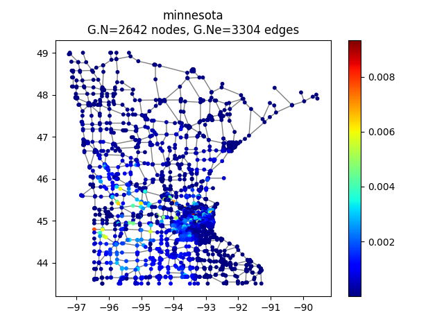
Look at the error between the original signal and its non linear approximation

>>> G.plot_signal(np.abs(Sig_iw_nT-Sig_iw),vertex_size=si)

../_images/Sig_nT_260_error_Minnesota.png

References¶

[cit1]

[cit2]

[cit4]