Run IntertwiningWavelet on other standard graphs: the sensor

We now use iw and run it on a standard graph: the sensor. We will study the multiresolution decomposition of a signal on this graph with iw and look at the approximation and detail components.

We will use the Toolbox PyGSP since it uses the weight matrix as a starting point to encode the graph, just as we do. We will use as well the visualization tools of PyGSP.

Feel free to use instead any of your favorite tool !

The Python File User_Example4.py can be downloaded to run the code of this tutorial. A function is required to write .g files and you find it in the file write_dot_g_sparse.py.

We start with a quick description of the outputs of the main class IntertwiningWavelet and show how to process a signal.

Getting started

Download modules

Load Python modules

The following Python modules should be useful.

• scipy.sparse since we will use sparse matrices,

• NumPy since we will process matrices and arrays,

• matplotlib.pyplot for visualization

>>> import numpy as np
>>> import scipy.sparse as sp
>>> import matplotlib.pyplot as plt

Load PyGSP modules

>>> from pygsp import graphs, filters, plotting

Load a module to write a .g file

We need a function to write from a matrix the .g file used by iw.

You can download here an example of such a function here write_dot_g_sparse.py (courtesy B. Stordeur). This works with a sparse adjacency matrix as it is the case with PyGSP.

>>> from write_dot_g_sparse import write_gsp_to_g

Load a graph

Graph input

Here we choose the sensor graph computed by PyGSP

>>> n=500
>>> G = graphs.Sensor(n, distribute=True, seed=42)

Graph visualization

We can have a look at it

>>> G.plot(vertex_size=50)

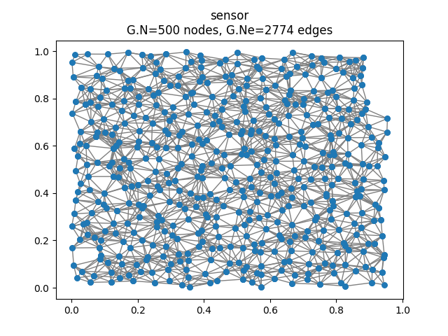
Sensor graph with 500 vertices.

Write the .g file

Remember iw runs with .g type files.

>>> W=G.W # Extract the weight matrix of the graph

>>> # write the .g file to run iw
>>> graph_g = 'sensor_test.g'
>>> write_gsp_to_g(W,graph_g)

Start the instances of IntertwiningWavelet

>>> from iw.intertwining_wavelet import IntertwiningWavelet
>>> iw = IntertwiningWavelet(graph_g)
"The graph is reversible the pyramide algorithm....
                can proceed"
>>> iw.pretreatment # To check if the graph has the required reversibility (symetry)
True

Run the method

Here we choose to have two levels of decomposition, i.e two levels of details. We could also decide the approximate number of the set of approximation coefficients.

>>> iw.process_analysis(mod='step', steps=2) # To have 2 levels of decomposition
>>> print(iw.process_analysis_flag) # True if the decomposition process has been done.
True
>>> tab = iw.tab_Multires # Attribute with all the analysis structure

Process a piecewise polynomial signal

We will now compute the intertwining wavelet (IW) coefficients of a piecewise polynomial signal defined and studied in [cit4] as well as in our article [cit2].

Signal input

>>> # Extract the coordinates of the vertex of the graph
>>> C=G.coords
>>> x=C[:,0]
>>> y=C[:,1]
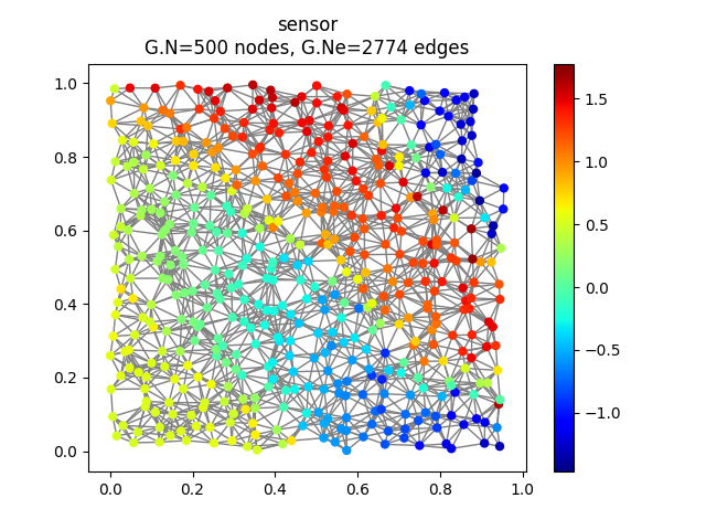
>>> Sig=np.where(y+x < 0.5,0.5+x**2+y**2, 0)
    +np.where(y+x<1.5,0.5+x**2+y**2,0)*np.where(y>1-x,1,0)
    +np.where(y>0.5-x,0.5-2*x,0)*np.where(y<1-x,1,0)+np.where(y>1.5-x,0.5-2*x,0)

Let us have a look on it

>>> plt.set_cmap('jet')
>>> G.plot_signal(Sig,vertex_size=25)

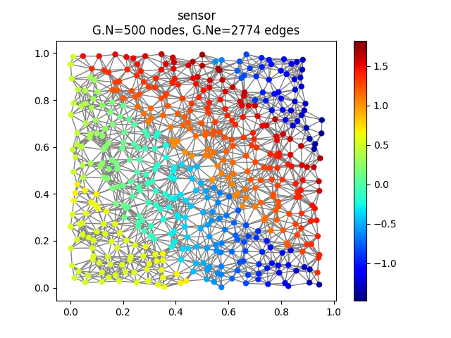
Original signal.

Computation of the intertwining wavelet coefficients

We compute the intertwining wavelet coefficients using the attribute of iw which is process_coefficients. The output is a 2d NumPy array, with possibly one line.

>>> # Reshape the signal to have it as a row matrix
>>> Sig_iw=np.reshape(Sig,(1,n))
>>> coeffs_iw = iw.process_coefficients(Sig_iw)

Organization of the coefficients:

The organization of the coefficients in the NumPy array coeffs_iw is as follows

coeffs_iw

with

• : the sequence of coefficients at the finest details level,

• : the sequence of coefficients at the coarsest details level,

• the sequence of scaling coefficients, or so called approximation coefficients.

The attribute following_size of iw gives the number of coefficients in each layer

>>> levels_coeffs = np.asarray(iw.following_size)
>>> print(levels_coeffs)
[188 126 186]

Remember our method is based on a random subsampling and thus the number of coefficients in each layer generally changes at each new run of iw. But we compute a basis and thus the total number of coefficients is always the total number of vertices in the graph.

In our example

• the finest details level has 188 coefficients,

• the coarsest details level has 126 coefficients

• we have 186 approximation coefficients in .

Visualization of the coefficients:

Watch out that the Intertwining basis is not orthonormal, and especially the basis vectors are not normalised. But we can anyway have a look at the coefficients.

>>> plt.figure()
>>> plt.plot(coeffs_iw[0,:])
>>> plt.title('IW coefficients')
>>> plt.show()

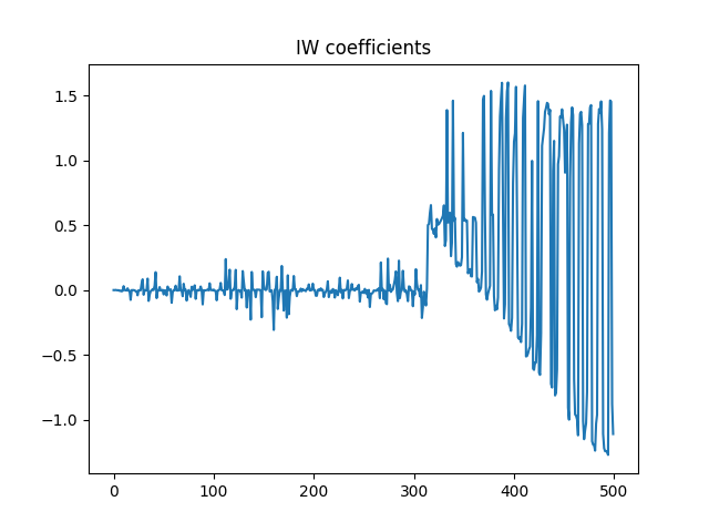
IW coefficients.

We can remark that the detail coefficients are much smaller than approximation ones.

Approximation and detail components

Our signal is the sum of three components: the approximation part, the finest detail part, the coarsest detail part. Let us have a look at each of these layers.

Approximation part

We reconstruct the signal whose wavelet coefficients are . This means that all the detail coefficients vanish.

>>> coeffs_approx_iw = np.zeros((1,n))
>>> napprox = levels_coeffs[tab.steps]

>>> # we keep only the f_2 coefficients.
>>> coeffs_approx_iw[0,n-napprox:n] = coeffs_iw[0,n-napprox:n].copy()

>>> # Let us have a look at it
>>> plt.figure()
>>> plt.plot(coeffs_approx_iw[0,:])
>>> plt.title('Coefficients of the iw approximation part')
>>> plt.show()

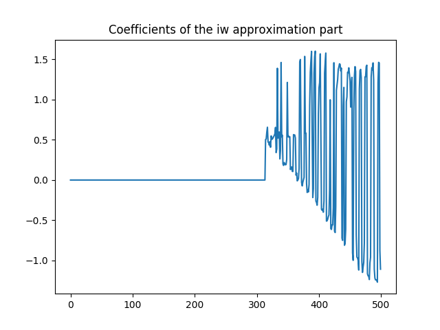
Approximation part coefficients computed with iw: only the 186 scaling coefficients are kept.

Let us compute the approximation part from its IW coefficients

>>> approx_iw = iw.process_signal(coeffs_approx_iw)

Let have a look at it

>>> G.plot_signal(approx_iw,vertex_size=25)

Approximation part with intertwining wavelets.

We remark it is smoother as the original signal, as we expected.

Finest detail part

We need to extract the first detail wavelet coefficients which corresponds to the finest detail coefficients.

>>> coeffs_detail1_iw = np.zeros((1,n))
>>> ndetail1 = levels_coeffs[0]

>>> # we keep the g_1 coefficients
>>> coeffs_detail1_iw[0,0:ndetail1] = coeffs_iw[0,0:ndetail1].copy()

Let us compute the finest detail contribution from its coefficients

>>> detail1_iw = iw.process_signal(coeffs_detail1_iw)

We visualize it

>>> G.plot_signal(detail1_iw,vertex_size=25)

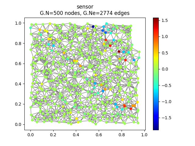
Finest detail contribution.

As we expect the finest detail part does not vanish at the discontinuities of the signal.

Coarsest detail part

We need to extract the coefficients corresponding to the coarsest detail level.

>>> coeffs_detail2_iw = np.zeros((1,n))
>>> ndetail2 = levels_coeffs[0]+levels_coeffs[1]

>>> # We keep the g_2 coefficients
>>> coeffs_detail2_iw[0,ndetail1:ndetail2] = coeffs_iw[0,ndetail1:ndetail2].copy()

Let us compute the coarsest detail contribution from its coefficients

>>> detail2_iw = iw.process_signal(coeffs_detail2_iw)

We visualize it

>>> G.plot_signal(detail2_iw,vertex_size=25)

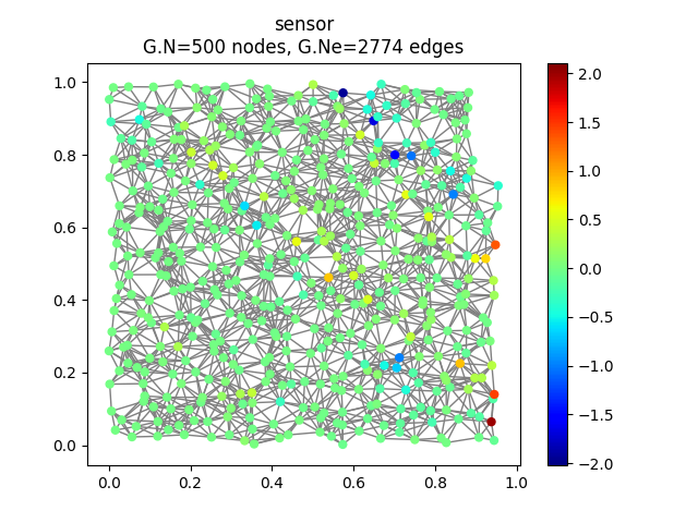
Coarsest detail contribution.

Signal reconstruction

The original signal should be the sum of these three layers. We compute the difference between this sum and the original signal.

>>> Sigr_iw = approx_iw+detail1_iw+detail2_iw
>>> G.plot_signal(Sig_iw-Sigr_iw,vertex_size=25)

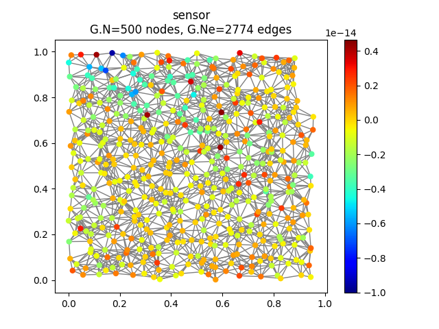
Difference between the original signal and its reconstruction as the sum of three layers.

We have a perfect reconstruction of the original signal using the sum of the three layers up to machine precision.

References

[cit1]

[cit2]

[cit4]